Note: All diagrams can be replicated through this python notebook (following soon), which includes the raw data (csv format) as well. Additionally some diagrams will feature their code below, so you can easily grab the example and adapt it to your dataset.

Context and main idea of this post

This blog post is a reflection on some group comparisons we did as part of the recently finished research project DOIT – Youth, social innovation, maker spaces and entrepreneurial education. We looked at more than 1.000 youths at the age between 6 and 16 in 10 different countries. There were many interacting concepts at play and each concept (e.g. the meaning of social innovation or entrepreneurship for kids under the age of 10) in itself was far from established in terms of what it meant and how it could be implemented best in the context of a pilots study. One of the questions the research addressed was

What impact does a minimum of 15 hours entrepreneurship-inspired, socially driven maker activities have on creativity and self-efficacy?

Both concepts - creativity and self-efficacy – were measure in a pre-post design. The tests themselves are explained in more detail here.

Yet, this short blog post is not about the semantic entanglement or definitional tensions a research project of this size is bound to generate, but about the statistical interpretation of the results we obtained and how they can be supported visually.

I include short definitions of the statistics used and see how visualizations can contribute to a better understanding of numerical results. We are using established python libraries for visualizations (e.g. seaborn or pyplot). Seaborn operates on top of pyplot and has a more declarative style, meaning that we focus on ’what it should show’ and less on ’how it can be shown’. However, this comfort comes with a caveat in that we need a sufficiently good understanding on how things are implemented under the hood to be competent judges of our own creations, i.e. does it really show what we want it to show. For example, as we will see, seaborn offers multiple parameters to support the visualization of a distribution including combinations of boxplots, histograms and kernel density estimations. While these combinations look more ‘fancy’ in general, they also use defaults which we need to be aware of for using them optimally.

Descriptive Statistics

Descriptive statistics include numerical summaries (e.g. mean, mode, standard deviation, interquartile ranges). The art of EDA (exploratory data analysis) which is also about visually inspecting the data, using tools such as histograms and scatter plots.

Note: I get some ideas from “Martin, O. (2018). Bayesian analysis with Python: Introduction to statistical modeling and probabilistic programming using PyMC3 and ArviZ. Packt Publishing Ltd.”, which is a fantastic book since it is a good reminder of the value of principle-driven thinking ...

Demographics

Since some of the group comparisons refer to gender and age, it’s good to get to know our data better in that respect. First, the sample is fairly balanced in terms of gender. We have two datasets: (a) one for self-efficacy testing (46% female participants) and (b) one for creativity testing (48% female participants). In general, we can assume that all participants did the self-efficacy and the creativity pre- and post-tests. You might wonder, why then the different sample sizes (n=759 versus n= 618 versus ...). The simple explanation is that not always all data had been collected. For example, in one instance an entire batch (about 50 participants) was returned without collecting the age. We still knew roughly their age group because of the class level they attended, so we could still use their data. The data records of individual learners from this quite distributed research design were up to 15% of reduced quality because core information (i.e. age, gender, hours participated in the program or test results) was lacking.

Before we can visualize data, a lot of efforts needs to go into collecting data in a standardized and consistent way.

Other types of data such as the professions of parents, was included in only 25.7 % of the responses. I think, we need to offer a convincing reason why we really need that information and make it mandatory, or else leave it out.

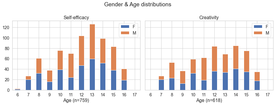
Age distribution: The younger age group (6 to 10 years) was about 27% and 29% in the two data samples. I think the age range is fairly broad, although the creativity test was based on drawings which seems much more inclusive of different ages and cognitive abilities, since creativity seems to be assessed more directly and doesn’t depend on other skills such as language and writing skills.

# data preparation
age_stacked_e = datae_sub [['Gender','Age']].groupby(['Age','Gender']).size()
age_stacked_c = datac_sub [['Gender','Age']].groupby(['Age','Gender']).size()

# creates enclosing figure (f) and two subplots (axs), sharing the y axis 
sns.set(rc={'figure.figsize':(13,5)}) 
sns.set( style='whitegrid', context='notebook', font_scale=1.3)
f, axs = plt.subplots(1, 2, sharey=True)
f.suptitle('Gender & Age distributions')

# plotting the bar charts 
axs[0].set_title('Self-efficacy')
age_stacked_e.unstack().plot.bar(stacked=True, ax=axs[0])
L=axs [0].legend()
L.get_texts()[0].set_text('F')
L.get_texts()[1].set_text('M')
plt.setp(axs[0].get_xticklabels(), rotation=0)
axs[0].set_xlabel('Age (n=' + str(len(datae_sub)) + ')')

axes[1].set_title('Creativity')
age_stacked_c.unstack().plot.bar(stacked=True, ax=axs[1])
L=axs [1].legend()
L.get_texts()[0].set_text('F')
L.get_texts()[1].set_text('M')
plt.setp(axs[1].get_xticklabels(), rotation=0)
axs[1].set_xlabel('Age (n=' + str(len(datac_sub)) + ')')

plt.tight_layout()

# subplotting: https://dev.to/thalesbruno/subplotting-with-matplotlib-and-seaborn-5ei8

Collinearity

Collinearity describes a redundance among the predictor variables or put differently some Independent variables correlate in a positive or negative way. While correlation between predictor and response is what we usually look for, collinearity between predictors needs to be corrected. (Note: We cannot tell the significance of one independent variable on the dependent variable if there is collinearity with another independent variable.) There are multiple scenarios how collinearity can emerge (e.g. data related, structure related, dummy variable trap).

Below we find a correlation-matrix. Numbers in each box show a correlation factor, where any relationship above 0.7 is interpreted as collinearity. There is actually little correlation happening, apart from ‘age’ correlating with ‘age group’ and ‘pre-test results’ correlating with post-test results’ (the labels are somewhat hidden by the color legend and refer to ‘PreTSDSummZf’ and ‘PostTSDSummZf’). The age and age group correlation is a classic case of ‘structural colinearity‘ since age group is only classifying ages into two categories (younger and older participants).

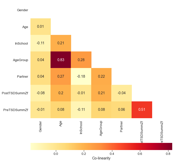
Note: In Python’s corr function uses pearson correlation coefficient as a standard, which measures the linear dependence between two variables. But you can also use kendall and spearman correlation methods for non-parametric, rank-based correlation tests.

sns.set(rc={'figure.figsize':(10,12)}) 
sns.set( style='whitegrid', context='notebook', font_scale=1.2)

def correlation_matrix (df): 
    correlations = df.corr().round(2)
    mask = np.zeros(correlations.shape, dtype=bool)
    mask[np.triu_indices(len(mask))] = True  #  indices for the upper-triangle of an (n, m) array.
    sns.heatmap(correlations, cmap="YlOrRd", annot=True, mask = mask, 
                cbar_kws={'label': 'Co-linearity', 'orientation': 'horizontal'})
    plt.show()

correlation_matrix (datac_sub)

Dealing with multicollinearity becomes increasingly relevant when doing regression modelling, there we can exclude correlating variables or do a principal components analysis. (Note: PCA is a common feature extraction technique reducing the dimensionality of data.)

Interventions: Duration of workshops and the age of facilitators

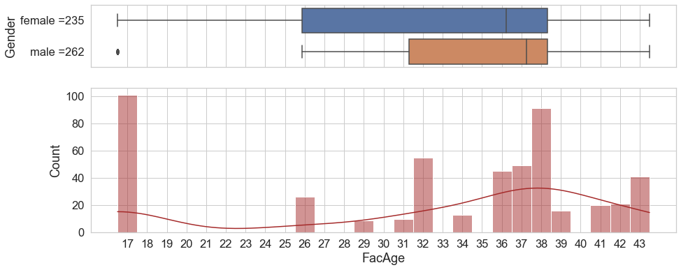
Beside age and gender of participants, we also have variables describing the educational programme, e.g. attended hours ranged from 15 to 43. Secondly, we know from other studies that gender and age of workshop facilitators – those implementing the intervention – can have an impact too. Hence plotting these dimension, e.g. their histogramms is a good first step.

Below we see three visualizations displaying the age of the facilitators in relaionship to workshop participants. We have a figure split in two parts, above a boxplot and below a histogram with a kernel density estimation. The boxplot shows that female participants had slightly younger facilitators than their male colleagues. The histogram highlights the huge group of facilitators at the age of 17 years, which is due to one partner implementing a workshop series based on peer-to-peer support. Lastly, the kernel density estimation indicates probable estimations for future values given the current sample.

And we can replicate the same visualization for ‘hours participated’ in workshops. Slightly more than half of the participants were engaged 15 or 16 hours. Male participants have a slightly lower median of hours engaged, but all in all we see little variation with 85% having between 15 und 21 hrs.

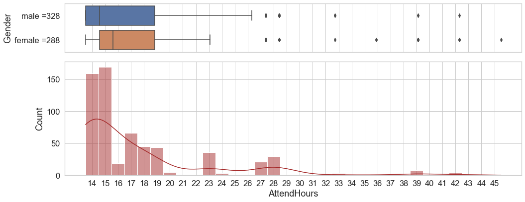
Note: Alligning the x-labels with the middle of each bar requires a bit of a hack, there might be an easier way. Also, the alignment doesn’t translate to the boxplot, so the markers at 28, 29 etc. , for example, are a bit off.

split =hours_attended.groupby('Gender').size()
females = 'female =' + str(split [0] )
males = 'male =' + str(split [1] )
print (females,males)

sns.set(rc={'figure.figsize':(15,6)})  
sns.set( style='whitegrid', context='notebook', font_scale=1.5)
f, (ax_box, ax_hist) = plt.subplots(2, sharex=True, gridspec_kw={"height_ratios": (.30, .70)})

xticks = np.arange(14, hours_attended['AttendHours'].max()+1)
plt.xticks(xticks)
ax_box = sns.boxplot(x =hours_attended['AttendHours'], data = facil_age, y = 'Gender', ax = ax_box  ).set(yticklabels=[males,females], xlabel='')
ax_hist = sns.histplot(data=hours_attended, x='AttendHours', bins = 32,  color = 'brown', kde = True, ax=ax_hist)

# calculate mid-point of bar and set correc label at this position 
mids = [rect.get_x() + rect.get_width() / 2 for rect in ax_hist.patches]
ax_hist.set_xticks(mids)
ax_hist.set_xticklabels(xticks)

plt.tight_layout()
plt.show()

Density estimations: Histograms, kernel functions and bandwidth parameters

Histograms are the most basic form of a probability estimation. Values, which are observed more often accumulate over time and show a higher bar in the chart. A critical point is often the binning, i.e. how many bars show an optimal representation.

Kernels can be thought of (not entirely correct) as weight functions for specific observations - data points -. The sum of all kernel probabilities makes the kernel density estimate. Wikipedia figures a very intuitive visualization:

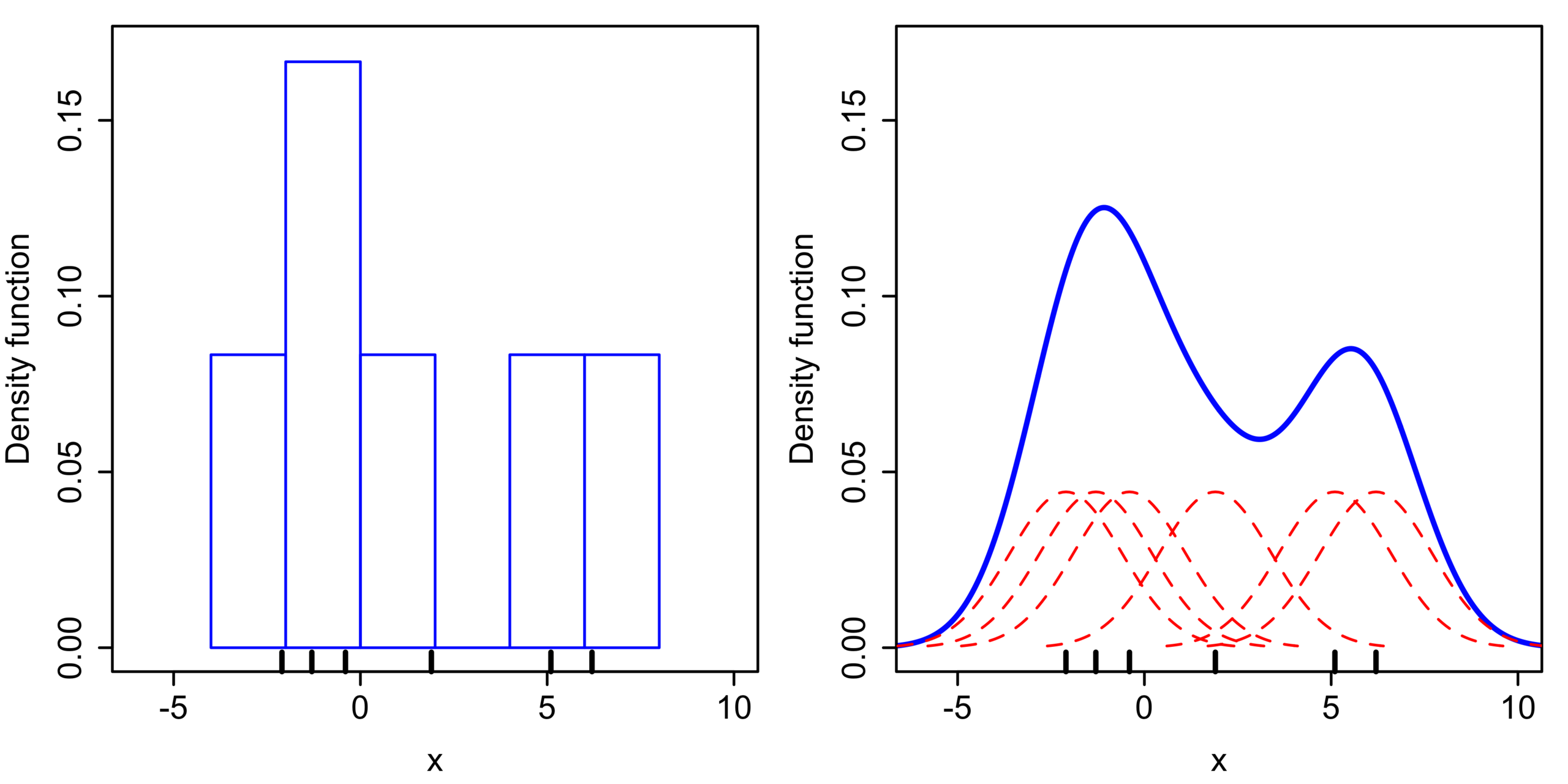
Estimate construction (https://en.wikipedia.org/wiki/Kernel_density_estimation)

What does it do?
Wikipedia: kernel density estimation (KDE) is a non-parametric way to generate the probability density function of a random variable. KDE is a data smoothing solution where inferences about the population are made, based on a finite data sample, that is, KDE is a method for using a dataset to estimate probabilities for new points.

Non-parametric basically means that the overarching probability distribution of a variable is not known and cannot be characterized by single parameters such as the mean or variance.(Note: expected probability and density are similar.)

More formally ... ‘What is a kernel?’. Kernel functions are used to estimate the density of a random variable and satisfy three properties:

they are symmetrical (max is in the middle, except for 'rectangular kernel functions'),
the area under the curve of the function must be equal to one,
K (kernel) values are always positive.

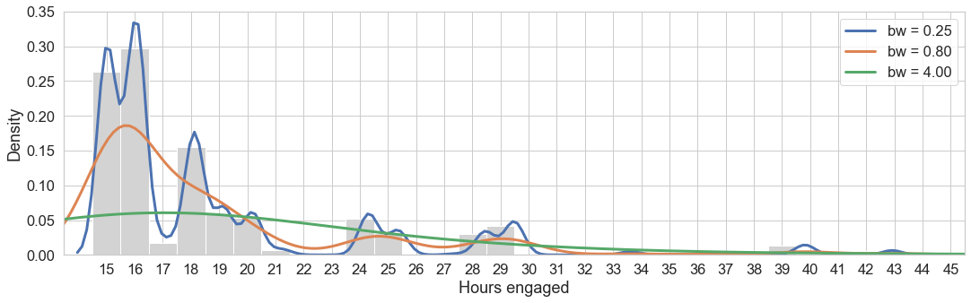
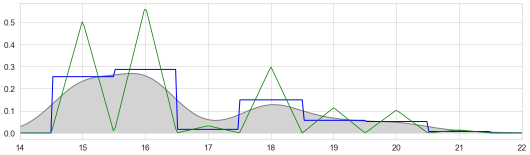
How smoothing our KDE graph looks like depends on our choice for the bandwidth parameter, which controls the number of samples or the window of samples used to estimate the probability for a new point. Below we see the density estimation for our example of ‘hours attended’. As a general rule, a too small bandwidth (e.g. bw = 0.25) shows too much variance (undersmoothing) and a too high bandwidth (e.g. bw = 4.00) hides much of the distribution characteristics, making the graph less useful. Below we see an overlay of histogram and three KDEs with different bandwith parameters to illustrate the resulting smoothing effects. For the purpose of visualizing a simple variable, you would go with the parameters the library would calculate in the background (e.g. bw≈0.8).

from sklearn.neighbors import KernelDensity
from scipy.stats import norm   
from numpy import asarray, exp

sns.set(rc={'figure.figsize':(18,5)}) 
sns.set( style='whitegrid', context='notebook', font_scale=1.5)

# x values for barchart and KDE graph  
sample = np.array(hours_attended)
sample2 = sample + 0.5
legend_items = []

# plotting the histogram 
sample = sample.reshape((len(sample), 1))
plt.hist(sample, bins=31, density=True, color='lightgrey') 

xticks = np.arange(15, hours_attended.max()+1)
plt.xticks(xticks)

# defining bandwidth parameters
bw = {
    'bw = 0.25':0.25,
    'bw = 0.80':0.8,
    'bw = 4.00':4
}

# plotting different KDEs 
for bw_key, bw_value in bw.items():
    g = sns.kdeplot(sample2, bw_adjust = bw_value, lw = 3) 
    legend_items.append(bw_key)

# styling: calculate mid-point of bar and set correct label at this position 
mids = [rect.get_x() + rect.get_width() / 2 for rect in g.patches]
g.set_xticks(mids)
g.set_xticklabels(xticks)

g.set_xlabel('Hours engaged')
g.set_ylabel('Density')
g.legend(labels=legend_items)

plt.xlim(14,45)    
plt.show()

#clearing lists prior to reruns 
mids.clear()
legend_items.clear()

However, KDE is an intersting approach with many potential applications: e.g. the exploratory analysis of point data for the recognition of geographical patterns - usually shown as heatmap - such as seismic risk estimation in earthquake areas. KDE is also needed for generative models, i.e. generating new point patterns for digits or faces. So I took the opportunity to dig a little bit deeper.

Beside bandwidth, kernel shapes / functions are an important parameter. Shown in Kernel Density Estimation, kernels can have many different shapes:

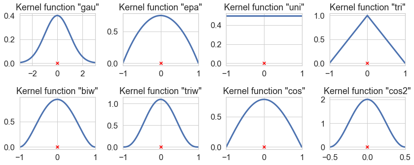
Bandwidth optimization is a whole different chapter ... Note: The way KDE is implemented depends on the libraries used: Scipy, Statsmodel and Scikit-Learn. For example, the seaborn KDE plot only supports the gaussian kernel. Analogue to the bandwidth discussion, we use the 'hours of workshop participation' dataset as an example, to demonstrate the effect of different kernel functions.

Comparing gaussian (grey), tophat (blue) and linear (green) kernels

T-test

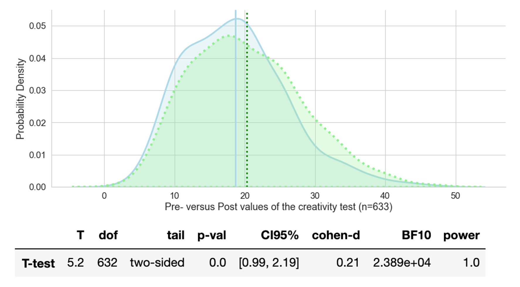
In an ideal (statistical) world, we would have two samples, both randomly selected with comparable backgrounds, one going through the educational program and another one being the control group. Below we can see two creativity test samples. The blue density curve, represents the results prior to the educational programme and the green one is the same group tested again after the programme. The t-test tells us that the means of the test results differ (statistically speaking) significantly and raise from 18.77 to 20.29. As always, significantly different simply means, being different with a very low probability that the observed difference is not explainable by chance alone. Going one step further, significant differences imply that the result should be repeatable.

Below the graph we have a table we can quickly go through. Concerning the first four pieces of information: we use a two-tailed t-test since the difference of means could be positive or negative. We could also use a one-tailed t-test if we were specifically interested in testing whether creativity de- or increases. Note: The two means are considered significantly different if the test statistic, i.e. the t-value, is in the top 2.5% or bottom 2.5% of its probability distribution, resulting in a p-value less than 0.05. or we can say ‘there is 95% confidence that the conclusion is valid’ - which also means that there is a 5% risk of being wrong.

The confidence interval (CI95%) indicates the two cut-off t-values, i.e. if the calculated t-statistics lies outside these boundaries, we can reject the null hypothesis (no group differences) in favour of the alternative hypothesis (groups are different). In the case above, T equals 5.2 and is well outside the 95% interval of the t-distribution, hence our participants show (we are not talking about causation) significantly improved results in the creativity test, after the educational programme. For demonstration purposes we could manipulate the creativity test results and say every participant gets one point less in the post-test (Note: the difference of means was 1.52). We would still have a significant improvement, but this time with a p-value of 0.05 and a much smaller T-value of 1.93, outside the new CI95% [-0.01, 1.19]. If, however, everybody would get 10 points more, the T-value would jump up to 37.9 (p=0.00).

T-value

We still need to explain the meaning of the T-value. A t-value is a ratio between the difference between two groups and the difference within the groups (i.e standard error). So if a t-value = obtained differences / standard error then T = 5.2 indicates that the observed difference is five times the size of the variability in our data.

Cohen’s d

We cannot assume that a significant effect is also a large effect. Cohen’s d =.21 is said to be a small effect and we can see that there is a huge overlap between the pre- and post results. Indeed, if we had a difference in means of 10 points, we would get Cohen’s d = 1.3.
From the calculation point of view it’s relatively straight forward, cohens_d = obtained differences / standard deviation. An excellent simulation shows how different d values translate into different overlaps of the estimated distributions represented by the two group means. The site also offers a ’common sense’ interpretation of d = 0.21 as we have it in our example.

With a Cohen's d of 0.21, 58.3% of the "treatment" group will be above the mean of the "control" group (Cohen's U3), 91.6% of the two groups will overlap, and there is a 55.9% chance that a person picked at random from the treatment group will have a higher score than a person picked at random from the control group (probability of superiority).

For the creativity tests, we used the following implementation ...

# calculating cohen's d manually 
from statistics import stdev

d = (mean_post_c - mean_pre_c) / ((stdev(post_c) + stdev(pre_c))/2)
d.round(2)
# => 0.21

What’s the difference between a t-value and Cohen’s d

Both values are ratios with the difference of means as numerators. The t-values puts this difference on relation to the standard error and Cohen’s d relates it to the standard deviation.

From a succinct description of the standard error and a helpful refresher from sample statistics’ we can take:

The standard deviation describes variability within a single sample and is a descriptive statistic (i.e., is calculated for a single sample). Visually, we could say if two normal distributions with the same mean, the distribution with the smaller standard deviation has the higher and narrower shaped bell curve.
The standard error estimates the variability across multiple samples of a population and is and inferential statistic (i.e., can only be estimated). By calculating the standard error, you can estimate how representative your sample is of your population. You can decrease standard error (and minimize sampling bias) by increasing the sample size or by increasing the realiability of the test eg. having more items in the questionnaire.

To sum up, t-values tell us about the general probability that two samples belong to different populations, i.e. given p = .05 we can assume with 95% certainty that group differences are not caused by chance. Once we have established that we are looking at two different populations, we calculate the ‘effect size’, based on the concrete standard deviations seen in the two samples.

Resources

Visualizations for Density Estimations and T-tests

Christian

Christian

Context and main idea of this post

Descriptive Statistics

Demographics

Collinearity

Interventions: Duration of workshops and the age of facilitators

Density estimations: Histograms, kernel functions and bandwidth parameters

T-test

T-value

Cohen’s d

What’s the difference between a t-value and Cohen’s d

Resources

T-Test

KDE

Simulations

Tableau: Five questions to check your visualizations

Hacking the knowledge of maker communities for Education

An empirically informed taxonomy for the Maker movement

How ‘new’ is the new Raspberry Pi Pico board?

Building the observation mapper